Problem 1: Loading Boxes into Different Types of Trucks.
To start, consider the following problem: 300 boxes need to be loaded and shipped to a warehouse from a factory. The logistics planner may rent trucks that can accomodate 40 boxes and 30 boxes, for RM 500 and RM 400. How many trucks of each type to minimize the cost?
Our goal is to minimize the cost of shipping these boxes by selecting the right amount of the different trucks.
Heuristic
This is a simple optimization problem. However, we don’t usually think in mathematical term while solving it. For many people, the answer is simple, even trivial. A box costs 12.50 for 40-boxes-truck and 13.33 for 30-boxes-truck. So we should prefer 40-boxes-truck to 30-boxes-truck. We first spend 3500 (7*500) for 7 40-boxes-truck and 280 boxes and then add an eighth 30-boxes-truck for 400 for the remaining 20 boxes. Total cost is RM 3900.
This looks fine. But this is not the best solution. With 6 trucks of 40 boxes (240 boxes and RM 3000) and 2 trucks with 30 seats (60 boxes and RM 800), we can ship the boxes and pay only RM 3800). We can save RM 100!
The best decision is not that obvious.
Graphical Method
Here is the summary of the information we have:
- We can use 2 kinds of trucks, which can accommodate **40 boxes and ***30 boxes*. We label them as truck40 and truck30 respectively.
- truck40 and truck30 are charged for RM 500 and RM 400 respectively.
- Our objective is to **minimize the cost, by allocating just enough trucks of different kinds.
- The total capacity from the trucks must be equal or more than the number of boxes, which is 300.
Let’s turn the information into mathematical representations.
- Minimize Cost = 500 truck40 + 400 truck30 – (1), (2) and (3)
- Boxes: 40 truck40 + 30 truck30 >= 300 – (4)
- truck40, bus30 >= 0
For the purpose of plotting, we need the co-ordinates of any 2 points from the above equation. In order to find the co-ordinates, simply insert a random value for either truck30 or truck40. Solving the equation after inserting the random values could then be used to find the value of the other coordinate.
For example, we can find the value of truck40 when truck30 = 0 by inserting zero in place of truck30 and solving the equation as follows:
Boxes: 40 truck40 + 30 (0) >= 300
40 truck40 + 0 = 300
40 truck40 = 300
truck40 = 300/40 = 7.5
So the coordinates of the first point are truck30 = 0 and truck40 = 7.5 which can be written as **(7.5, 0).
Similarly, we can find the value of truck30 when truck40 = 0 by inserting zero in place of truck40:
Boxes: 40 (0) + 30 truck30 >= 300
0 + 30 truck30 = 300
30 truck30 = 300
truck30 = 300/30 = 10
So the coordinates of the second point are truck40 = 0 and truck30 = 10 which can be written as **(0, 10).
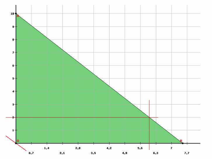
Once we have determined the coordinates of any 2 points from the equation, we simply mark them on the graph and draw a straight line across them.
We shade the area on graph which lies on or below the linear equation line.

We can now calculate the cost for these two points.
Cost = 500 truck40 + 400 truck30
For point A (0, 10):
Cost = 500(0) + 400(10) = RM 4000
Not bad! How’s about point B?
For point B (7.5, 0):
Cost = 500(7.5) + 400(0) = RM 3750
Better! Lower cost! So, we just need 7.5 trucks that can accommodate 40 boxes each.
Linear Programming (LP)
Linear programming is the best known mathematical optimization technique where we depict complex relationships through linear functions and then find the optimum points. It is a method to allocate scarce resources to competing activities in an optimal manner when the problem can be expressed using a linear objective function and linear inequality constraints.
George Dantzig, the father of linear programming, invented Simplex method in 1947. Simplex method is an iterative procedure to keep transforming the value of basic variables to get the most feasible solution for the objective function. It is the first generalized algorithm for solving linear programming problem and the basis for many optimization algorithms.
George Dantzig & W. Orchard-Hays revised it in 1953 to improve the efficiency of Simplex algorithm. The algorithm starts somewhere along the edge of the shaded feasible region and travels from vertex to vertex until arriving at the vertex that also intersects the optimal objective line (optimal solution). The vertex with the optimal objective value is the one that intersects the isoprofit line (extreme point of the feasible region).
To solve a linear optimization problem, a model file usually contains the following elements:
1) Decision Variables are the best values of the variables to solve a problem. Decision variables must be continuous, i.e. x E [-1,1] (cannot be discrete, i.e. x E (0,1). In our case, they are the different kinds of trucks, i.e. truck40 and truck30. They are the best solution when they are 6 and 2 respectively.
2) Objective Function is the objective of a linear programming problem, which will be to maximize or to minimize some numerical value. In our case, our objective is to minimize the cost. At the end, we just need to pay RM 3800, instead of RM 4000.
3) Linear Constraints typically represent resource constraints or the minimum or maximum level of some activity. They define the possible values the variables of a linear programming problem may take. They are expressed as equalities or inequalities with linear expressions on either side. Inequalities must be of the form >= or <=. No restrict inequalities (> or <) allowed. In our case, we need to make sure we will have enough capacity for all 300 boxes.
4) Non-negativity restriction is a special kind of constraint. For all linear programs, the decision variables should always take non-negative values, which are greater than or equal to 0. In our case, the number of trucks are 0 or more, never negative.
5) Feasible Region is the set of all points that satisfy all the constraints. One of them will be our optimal solution point.
Here is the conventional form or typical symbolic representation of a LP.
Minimize (or Maximize)
 c1 x1 + c2 x2 + ... + cn xn

Subject To
 a11 x1 + a12 x2 + ... + a1n xn ~ b1
 a21 x1 + a22 x2 + ... + a2n xn ~ b2
 ...
 am1 x1 + am2 x2 + ... + amn xn ~ bm
 x1, x2, ... , xn >= 0

Bounds
 l1 <= x1 <= u1, ... ln <= xn <= un
- relation ~ in inequalities form (>=, <=)
- objective function coefficients c1, …, cn
- constraint coefficients a11, …, amn
- righthand side b1, …, bm
- upper bounds u1, …, un
- lower bounds l1, …, ln
- variables or unknowns x1, …, xn
Short form
min c x
s. t. Ax >= b
x >= 0
- model starts with the objective, i.e. to minimize a linear function x; c = vector of objective coefficients
- subject to constraints in the form of linear expressions; b is the vector of right-hand side constants of constraints; A is the matrix of constraint coefficient; x is the decision variable
- variable domain (>=0)
More: Optimization Model Development and Mathematical Techniques for Optimized Solution
Problem 1 Revisited
The truck company can only rent the whole truck. We cannot rent a 0.5 truck. It has to be a whole truck, leaving the empty space unoccupied. So, based on our graph, we will have to go for the 10 30-boxes-trucks with the cost of RM 4000.
If you really think so, you are leaving money on the table! Any point under the shaded area is the possible solution. Luckily, not many are integer coordinates, i.e. a pair of integer numbers.
To find the optimum point, we need to slide a ruler across the graph. To minimize the cost, we must slide the ruler up to the point within the area that is nearest to the origin.

We find that point (6, 2) is an integer pair.
Cost = 500 bus40 + 400 bus30
For point (6, 2):
Cost = 500(6) + 400(2) = RM 3800
So, we actually need 6 40-boxes-trucks and 2 30-boxes-trucks to get the lowest cost.
Integer Programming
It is actually a more specific case of linear programming problem, called Integer Linear Programming (ILP). Integer Programming is a subset of Linear Programming. It has all the characteristics of an LP, an attempt to find a maximum or minimum solution to a function given certain constraints, except for one caveat: the solution to the LP must be restricted to integers. According to the nature of the variables, we can distinguish three types of IP models, which are Pure IP (as our example here), Mixed IP and Binary IP.
The Problem 1 is a simple example with only 2 variables, which are 2 kinds of trucks. In reality, real business problems in real companies can contain up to thousands or more variables. Solving it graphically is totally impossible. With modern tools, like CPLEX, companies can tackle more complex real-world problems and the return of investment would not be just RM 100 as in our toy truck problem but millions of dollars. In the next blog, we will revisit this problem using CPLEX/OPL.